WSPR vs CW SNR Comparison
Here I try to explain how to compare WSPR (Weak Signal Propagation Reporter) measurements with CW (Morse Code) to determine if a signal path is viable for a contact.
1. Some Math
WSPR’s advantage over CW comes from two distinct mathematical sources: Bandwidth Gain and Coding Gain.
A. Bandwidth Gain (The Filter Effect)
The noise floor is directly proportional to bandwidth (drops as the bandwidth narrows). By narrowing the window, we exclude noise.
- Calculation: 10 * log10(BW_Reference / BW_WSPR)
- Reference (SSB): 2500 Hz
- WSPR Bandwidth: ~6 Hz
- Gain: 10 * log10(2500 / 6) ≈ 26.2 dB
Impressive in case of SSB, so let’s see CW:
- CW Bandwidth: ~500 Hz (Standard filter, I know we may go down to 50 Hz 😎)
Gain: 10 * log10(500 / 6) ≈ 19.2 dB
B. Coding Gain (The Digital Magic)
Unlike CW, which relies on the human brain to “match” patterns, WSPR uses Forward Error Correction (FEC). It sends 162 bits of data to convey only 50 bits of actual information.
- The Formula: G_coding = Eb/N0_unencoded - Eb/N0_encoded
- For the convolutional code used in WSPR, the effective Coding Gain is approximately 4 to 5 dB.
2. The K=32 Convolutional Code
The “secret sauce” of WSPR is its extremely long constraint length, K=32.
In digital communications, the constraint length (K) defines how many previous bits influence the current encoded bit. While many modes (like NASA’s Voyager) used K=7 or K=9, WSPR uses K=32.
Why K=32 Matters:
- Redundancy: WSPR uses a rate r=1/2 convolutional code. This means for every bit of data, two bits are transmitted.
- Complexity vs. Performance: A larger K provides a steeper “waterfall curve” in performance, meaning the transition from “no copy” to “perfect copy” happens over a very small SNR range.
- The Fano Algorithm: Because a K=32 code is too complex for standard Viterbi decoding (which would require 2^{31} states), WSPR uses the Fano Algorithm. This is a sequential decoding process that searches through a “tree” of possible bit sequences, back-tracking when it hits a path that is too noisy.
This coding allows WSPR to function at an Eb/N0 (Energy per bit / Noise power spectral density) of only about 1 to 2 dB, whereas CW typically requires significantly more signal energy to be intelligible.
3. Mode Sensitivity Comparison
All values are referenced to a 2500 Hz standard bandwidth.
| Mode | Min. SNR | Bandwidth Gain | Coding Gain | Total Adv. vs SSB |
|---|---|---|---|---|
| SSB Voice | +10 dB | 0 dB | 0 dB | 0 dB |
| CW 🎧 | -10 dB | ~7-10 dB* | 0 dB | 20 dB |
| WSPR | -29 dB | 26.2 dB | ~4 dB | 30.2 dB |
*CW bandwidth gain varies based on the operator’s mental “filter”.
4. Power Increase for CW
WSPR is usually run at QRPP levels (I use 200 mW). Comparing the detection thresholds of the two modes in a standard 2500 Hz bandwidth:
- WSPR Threshold: WSPR can be decoded down to -29 dB to -31 dB.
- CW Threshold: A human operator requires an SNR of roughly -10 dB to copy Morse code reliably (500 Hz filter, 15-20 WPM).
That means:
(-10 dB [CW]) - (-30 dB [WSPR]) = 20 dB difference.
To make a signal that WSPR just barely sees (-30 dB) audible for a human (-10 dB), I have to increase my TX power by a factor of 100 (!). 💪
| If WSPR Power is… | To get the same “Readability” on CW, I need… |
|---|---|
| 100 mW | 10 Watts |
| 200 mW | 20 Watts |
| 500 mW | 50 Watts |
| 1 Watt | 100 Watts |
| 5 Watts | 500 Watts |
5. Practical Rule of Thumb
While technically, the difference between the WSPR threshold and the average CW threshold is 20 dB. However, for a practical “Rule of Thumb,” I use a 2 dB “Safety Margin” and thus 18 dB because of:
- QSB (Fading Penalty (-3 to -5 dB)): WSPR integrates a signal over nearly 2 minutes. It can “ride out” deep fades that would cause me in a CW QSO to lose a character or more.
- The Human Bonus (+5 dB): While a “standard” operator like me needs -10 dB, an expert ear can often copy signals down to -15 dB if the signal is steady.
- The Result: These factors almost cancel out. I use 18 dB as a conservative “safe bet” so that if the math says the path is open, the QSO actually happens.
So if I have a WSPR report and want to know if I could have made that contact via CW at the same power level, I use 18 dB to ensure that if the math says “it’s possible,” I actually have a high probability of success despite fading and noise bursts.
The Formula
WSPR_SNR + 18 dB = Estimated_CW_SNR
Examples
-
Case A (Strong Path): I receive a WSPR spot of -10 dB.
-10 dB + 18 dB = +8 dB
Result: The signal is 18 dB above the CW threshold. A QSO would be very easy at current power. 🙂 -
Case B (Weak Path): I receive a WSPR spot of -25 dB.
-25 dB + 18 dB = -7 dB
Result: This is audible but weak. I could make the contact, but it would require focus. 🤨 -
Case C (Limit): I receive a WSPR spot of -30 dB.
-30 dB + 18 dB = -12 dB
Result: This is below my hearing threshold. I would likely need to increase my power by at least 10 dB to be heard on CW. ☹️
6. Summary
The takeaway from all this is: If my WSPR spots are -18 dB or better, the path is open and on top there is a feasibility of QRPP CW.
If my WSPR reports (transmitted at 200 mW) are consistently -18 dB or better, the SNR math predicts my signal would be roughly 0 dB in a standard CW bandwidth. This is a clear, “armchair copy” signal, thus I have a very high probability of completing a CW contact on that same path using the very same 200 mW. 🤩 While the math is solid, two non-mathematical hurdles remain for low-power CW:
- The Other Station’s Noise Floor: My above SNR calculations assume a “standard” noise floor. If the receiving station has high local QRN, they will not hear my 200 mW signal regardless of the ionospheric opening. 😥
- The Human Coordination Factor: Unlike WSPR, where the spotters are always listening, CW requires a human to be tuned to my frequency at the exact moment I call ‘CQ’ …
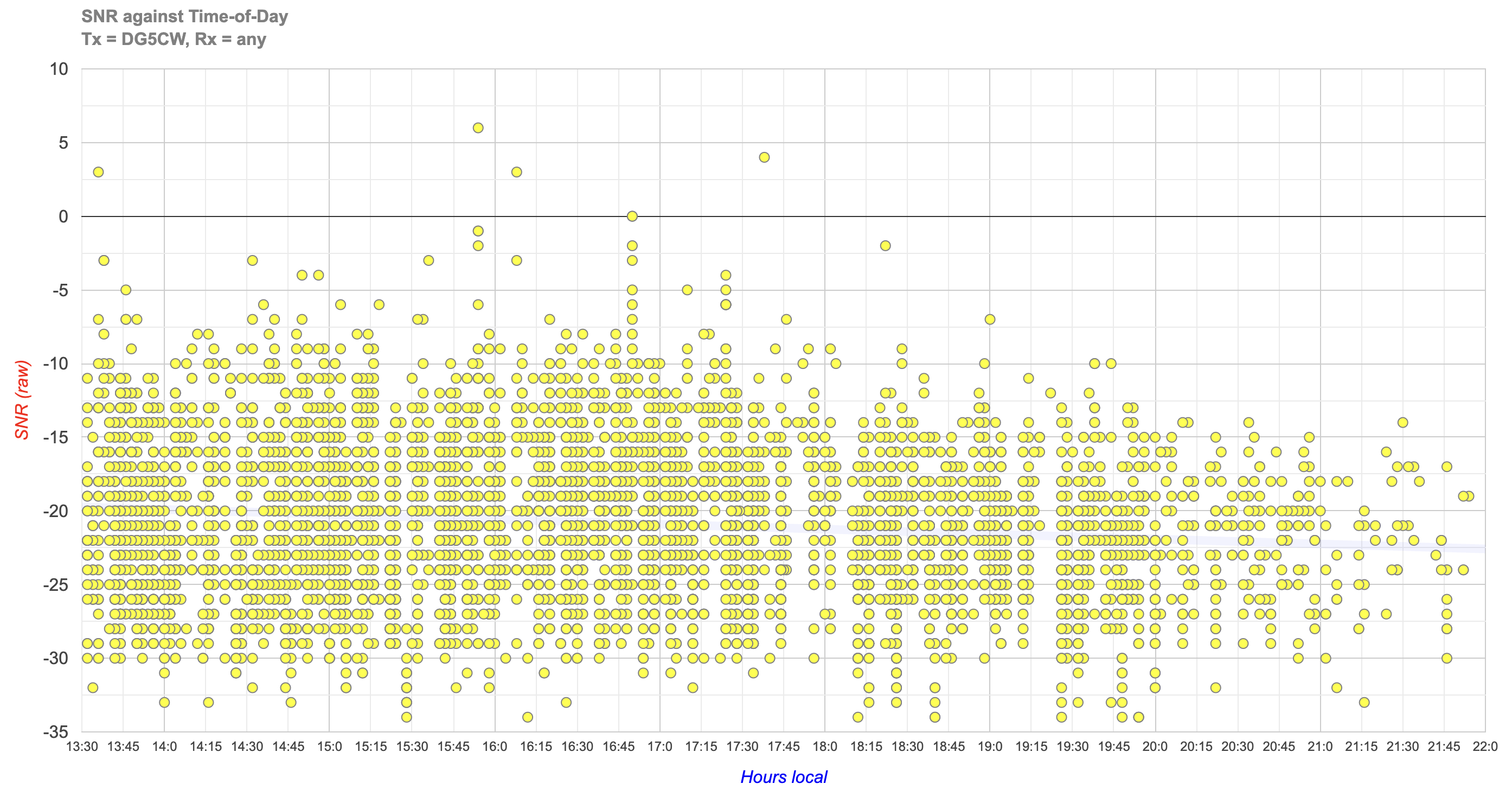
Above: SNR against time of the day for my 40m band mini dipole.